Decision trees and random forests, explained simply

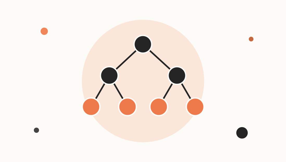
A decision treeA model that predicts by asking a chain of yes/no questions about the input, like a flowchart is the one machine learning model you can read out loud. It is also the building block of random forests and gradient boosting, which win a huge share of real-world tabular-data problems. This guide explains how a tree chooses its questions, why it overfits, and how a forest repairs that.

A tree is just a flowchart

Here is a tree trained on the classic iris flower data, printed by scikit-learn:

|--- petal width (cm) <= 0.80
|   |--- class: 0
|--- petal width (cm) >  0.80
|   |--- petal width (cm) <= 1.75
|   |   |--- class: 1
|   |--- petal width (cm) >  1.75
|   |   |--- class: 2

To classify a flower you start at the top and follow the answers: is the petal narrower than 0.8 cm? If yes, species 0. Otherwise, is it narrower than 1.75 cm? — and so on until you reach a leaf. No equations, no scaling, no black box.

You can produce this yourself:

from sklearn.datasets import load_iris
from sklearn.tree import DecisionTreeClassifier, export_text

iris = load_iris()
tree = DecisionTreeClassifier(max_depth=2, random_state=0)
tree.fit(iris.data, iris.target)

print(export_text(tree, feature_names=iris.feature_names))

How does the tree choose its questions?

At every node the tree tries many possible splits ("is feature f ≤ threshold t?") and keeps the one that makes the resulting groups purest. A group is pure when it contains mostly one class.

The usual measure is Gini impurityA score from 0 (all one class) upward measuring how mixed a group is:

gini = 1 - sum(p_class ** 2)

where p_class is the share of each class in the group.

A worked example

A node holds 10 customers: 6 bought, 4 did not.

gini = 1 - (0.6² + 0.4²) = 1 - (0.36 + 0.16) = 0.48

Try splitting on "visited the pricing page":

• Left group: 6 customers, 5 bought, 1 did not → 1 - (5/6)² - (1/6)² = 0.278
• Right group: 4 customers, 1 bought, 3 did not → 1 - (1/4)² - (3/4)² = 0.375

The weighted average impurity after the split is:

(6/10) × 0.278 + (4/10) × 0.375 = 0.317

The split reduced impurity from 0.48 to 0.317, a gain of about 0.163. The tree computes this for every feature and threshold and picks the biggest gain. Then it repeats inside each child. That is the entire algorithm: greedy, recursive purity-chasing.

Why one tree overfits

Left alone, a tree keeps splitting until every leaf is pure — which can mean one leaf per training example. It memorises. On the breast-cancer dataset:

from sklearn.datasets import load_breast_cancer
from sklearn.model_selection import train_test_split
from sklearn.tree import DecisionTreeClassifier

X, y = load_breast_cancer(return_X_y=True)
X_train, X_test, y_train, y_test = train_test_split(
    X, y, test_size=0.25, random_state=42, stratify=y
)

for depth in [None, 3]:
    tree = DecisionTreeClassifier(max_depth=depth, random_state=42)
    tree.fit(X_train, y_train)
    print(depth, tree.score(X_train, y_train), tree.score(X_test, y_test))

Typical results:

The unlimited tree scores a perfect 100% on data it has seen and worse on new data. That gap is overfitting. Limiting depth (or min_samples_leaf) is called pruning and trades a little training accuracy for better generalisation.

Trees are also unstable: change a few training rows and the top question can change, producing a completely different tree. That instability is the key to the next idea.

Random forests: many trees, one vote

A random forestAn ensemble of many decision trees, each trained on a different random sample, whose predictions are averaged trains hundreds of trees and lets them vote. To make the trees different (voting on identical trees is pointless) it adds two kinds of randomness:

1. Bootstrap sampling. Each tree trains on a random sample of the rows, drawn with replacement, so it sees a slightly different dataset.
2. Random feature subsets. At each split, only a random handful of features are considered, so trees cannot all copy the same strongest question.

Each tree overfits in its own way. Averaging 200 of them cancels most of the individual noise while keeping the signal. This idea of reducing variance by averaging is called bagging.

from sklearn.ensemble import RandomForestClassifier

forest = RandomForestClassifier(n_estimators=200, random_state=42)
forest.fit(X_train, y_train)

print(forest.score(X_train, y_train))   # 1.0
print(forest.score(X_test, y_test))     # about 0.96

On this split the forest reaches about 96% test accuracy against 92% for the unlimited single tree — better, without any tuning. (Exact numbers shift with the split; run it on several seeds before drawing conclusions. Cross-validation gives you a steadier estimate.)

Which features mattered?

Forests report how much each feature reduced impurity across all trees:

from sklearn.datasets import load_breast_cancer

names = load_breast_cancer().feature_names
ranked = sorted(zip(forest.feature_importances_, names), reverse=True)[:5]
for score, name in ranked:
    print(f"{score:.3f}  {name}")

For this data the top features are measurements like worst perimeter, worst area and worst concave points. Treat importances as a hint, not proof: they favour features with many distinct values and can split credit between correlated features.

The settings that matter

Strengths and weaknesses

Good at: mixed numeric and categorical-style data, no scaling needed, captures non-linear patterns and feature interactions, hard to badly misconfigure.

Weak at: extrapolating beyond the range of training data (a tree can only output values it has seen), very high-dimensional sparse data like raw text, and giving a model small enough to read — a 200-tree forest is not interpretable the way one tree is.

FAQ

How does a decision tree decide where to split?

It tests many candidate questions and picks the one that makes the child groups purest, usually measured by the drop in Gini impurity or entropy. It then repeats on each child.

Why is a random forest better than a single decision tree?

A single tree overfits and changes a lot with small data changes. A forest averages many different trees, which cancels their individual errors and generalises better.

Do decision trees need feature scaling?

No. Splits compare a feature to a threshold, so standardising or normalising the data changes nothing.

How many trees should a random forest have?

Start with 100–200. Accuracy usually plateaus, so more trees mainly cost time. Check that the score stops improving rather than guessing.

Next reading on Sythra Articles

• Cross-validation: why one train/test split lies
• How to detect overfitting
• Your first machine learning model with scikit-learn