Backpropagation worked out with real numbers

BackpropagationThe algorithm that computes how much each weight contributed to the error, using the chain rule from the output backwards is usually explained with symbols until your eyes glaze. Here we do the opposite: one tiny network, one training example, every number written out. By the end you will see that backprop is just the chain rule applied in a sensible order, and you will have code that proves the hand calculation right.

The network

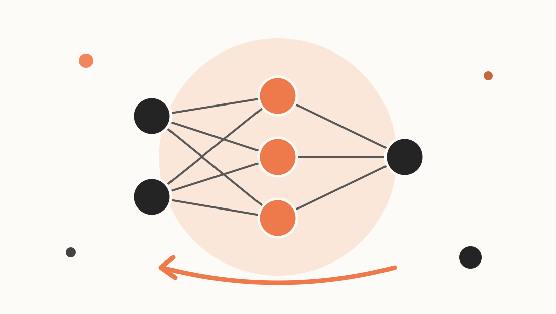
Two inputs, two hidden neurons, one output. All neurons use the sigmoid function; there are no biases, to keep the arithmetic short.

 input         hidden         output

  x1 ──┬──────► h1 ──(w5)──┐
       │   ╲  ╱            ├──► o
  x2 ──┴──────► h2 ──(w6)──┘

  every input connects to every hidden neuron (the four W1 weights)

The sigmoidA smooth function that squashes any number into the range 0 to 1 and its derivative:

σ(z)  = 1 / (1 + e^-z)
σ'(z) = σ(z) · (1 − σ(z))

That derivative formula is the convenient fact that makes the algebra short: we can reuse the output we already computed.

Starting values:

x  = [0.5, 1.0]          target y = 1.0
W1 = [[0.1, 0.3],        # W1[i][j] connects input i to hidden neuron j
      [0.2, 0.4]]
W2 = [0.5, 0.6]          # hidden neuron j to the output
loss L = ½ (o − y)²

Forward pass

Hidden pre-activations (z = x · W1):

z_h1 = 0.5·0.1 + 1.0·0.2 = 0.25
z_h2 = 0.5·0.3 + 1.0·0.4 = 0.55

Hidden activations:

h1 = σ(0.25) = 0.5622
h2 = σ(0.55) = 0.6341

Output:

z_o = 0.5622·0.5 + 0.6341·0.6 = 0.6616
o   = σ(0.6616) = 0.6596

Loss:

L = ½ (0.6596 − 1.0)² = 0.0579

The network predicts 0.66 where we wanted 1.0. Now: how should each weight change to close that gap?

Backward pass

We want ∂L/∂w for every weight. The chain rule says: multiply the local derivatives along the path from the loss back to that weight. Work from the output toward the inputs, reusing earlier results.

Step 1 — Loss to output

∂L/∂o = o − y = 0.6596 − 1.0 = −0.3404

Negative: the output is too low, so increasing it reduces the loss.

Step 2 — Through the output sigmoid

∂L/∂z_o = ∂L/∂o · σ'(z_o)
        = −0.3404 · 0.6596 · (1 − 0.6596)
        = −0.0764

Call this value δ_o. Everything upstream builds on it.

Step 3 — Output-layer weights

z_o = h1·w5 + h2·w6, so the derivative of z_o with respect to each weight is simply the hidden activation feeding it:

∂L/∂w5 = δ_o · h1 = −0.0764 · 0.5622 = −0.0430
∂L/∂w6 = δ_o · h2 = −0.0764 · 0.6341 = −0.0485

Step 4 — Send the error back to the hidden layer

How much did each hidden neuron contribute to the output error? Weight the error by the connection strength:

∂L/∂h1 = δ_o · w5 = −0.0764 · 0.5 = −0.0382
∂L/∂h2 = δ_o · w6 = −0.0764 · 0.6 = −0.0459

This is the step that gives backpropagation its name: the error signal travels backwards along the same weights the forward pass used.

Step 5 — Through the hidden sigmoids

δ_h1 = ∂L/∂h1 · h1(1 − h1) = −0.0382 · 0.5622 · 0.4378 = −0.00941
δ_h2 = ∂L/∂h2 · h2(1 − h2) = −0.0459 · 0.6341 · 0.3659 = −0.01064

Step 6 — First-layer weights

Each weight's gradient is the delta of the neuron it feeds, times the input it carries:

∂L/∂W1[0][0] = δ_h1 · x1 = −0.00941 · 0.5 = −0.00470
∂L/∂W1[0][1] = δ_h2 · x1 = −0.01064 · 0.5 = −0.00532
∂L/∂W1[1][0] = δ_h1 · x2 = −0.00941 · 1.0 = −0.00941
∂L/∂W1[1][1] = δ_h2 · x2 = −0.01064 · 1.0 = −0.01064

Notice how small these are compared with the output-layer gradients. Each sigmoid multiplied the signal by a factor of at most 0.25. Stack many layers and the gradient shrinks toward zero — the vanishing gradient problem, and a big reason modern networks prefer ReLU-style activations.

The update

Gradient descent subtracts the gradient times a learning rate. With lr = 0.5:

w5 = 0.5 − 0.5·(−0.0430) = 0.5215
w6 = 0.6 − 0.5·(−0.0485) = 0.6242
W1[0][0] = 0.1 − 0.5·(−0.00470) = 0.10235
... and so on

Every gradient was negative, so every weight rose, pushing the output upward toward 1.0. After the update, re-running the forward pass gives o ≈ 0.6661 and L ≈ 0.0557 — down from 0.6596 and 0.0579. One step, a measurable improvement.

Prove it in NumPy

import numpy as np

def sigmoid(z):
    return 1 / (1 + np.exp(-z))

x = np.array([0.5, 1.0])
y = 1.0
W1 = np.array([[0.1, 0.3], [0.2, 0.4]])
W2 = np.array([0.5, 0.6])

# forward
z1 = x @ W1
h = sigmoid(z1)
z2 = h @ W2
o = sigmoid(z2)
loss = 0.5 * (o - y) ** 2
print("forward:", h, o, loss)

# backward
d_o = o - y
delta_o = d_o * o * (1 - o)
dW2 = delta_o * h

d_h = delta_o * W2
delta_h = d_h * h * (1 - h)
dW1 = np.outer(x, delta_h)

print("dW2:", dW2)
print("dW1:", dW1)

# update
lr = 0.5
W1 -= lr * dW1
W2 -= lr * dW2

o_new = sigmoid(sigmoid(x @ W1) @ W2)
print("new loss:", 0.5 * (o_new - y) ** 2)

The printed gradients match the hand calculation. Two lines of the backward pass carry the entire idea:

• delta_o — the error at a neuron after passing back through its activation
• d_h = delta_o * W2 — the error pushed backwards through the weights

Check your gradients numerically

Whenever you derive gradients yourself, verify them. A gradient check nudges one weight by a tiny amount and measures the real change in loss:

def loss_fn(W1, W2):
    o = sigmoid(sigmoid(x @ W1) @ W2)
    return 0.5 * (o - y) ** 2

W1 = np.array([[0.1, 0.3], [0.2, 0.4]])
W2 = np.array([0.5, 0.6])
eps = 1e-6

W2_plus = W2.copy();  W2_plus[0] += eps
W2_minus = W2.copy(); W2_minus[0] -= eps
numeric = (loss_fn(W1, W2_plus) - loss_fn(W1, W2_minus)) / (2 * eps)
print(numeric)    # about -0.04296, matching dW2[0]

If the numeric and analytic values disagree beyond a few decimal places, there is a bug in your backward pass. This is the standard way people debug hand-written networks.

What this scales to

Real frameworks do exactly this, automatically:

• PyTorch's loss.backward() records every operation in the forward pass, then walks the graph in reverse applying the chain rule.
• Matrices replace single numbers, so delta * h becomes a matrix product like the ones in our matrix operations guide.
• The structure is identical in a CNN or a transformer.

Once you have seen one step with real numbers, backward() stops being magic.

FAQ

What is backpropagation in simple terms?

Backpropagation computes how much each weight in a neural network contributed to the final error. It applies the chain rule from the output layer backwards, reusing intermediate results, so all gradients come out in one backward sweep.

Why is it called backpropagation?

Because the error signal flows backwards through the network, from the output toward the inputs, along the same connections the forward pass used.

What is the vanishing gradient problem?

When gradients pass through many layers of saturating activations like sigmoid, each layer multiplies them by a small number, so early layers receive almost no learning signal. ReLU activations, residual connections and good initialisation reduce this.

How do I know my gradients are correct?

Run a numerical gradient check: nudge a weight by a tiny epsilon, measure the change in loss, and compare with your analytic gradient. They should agree to several decimal places.

Next reading on Sythra Articles

• Linear regression from scratch with NumPy
• A CNN from scratch in NumPy
• Transformer from scratch in PyTorch